Thomas Schlitt
A short introduction to molecular biology
menu:
A quick introduction to elements of biology - cells, molecules, genes, functional genomics, microarrays
Alvis Brazma, Helen Parkinson, Thomas Schlitt, Mohammadreza ShojatalabDraft, October 2001
This is a brief introduction to molecular biology with emphasis on genomics and bioinformatics. It is intended for scientists, engineers, computer programmers, or anybody with background or strong interest in science, but without background in biology. I was originally written first of all for those scientists, engineers, etc. joining the EBI. On one hand we have tried to distil the content down to the absolute minimum needed to make some sense of bioinformatics, while on the other to leave in enough to show why it is interesting.
Content
1. Organisms and cells
2. Molecules of life
3. Genes and genomes
4. Functional genomics
5. Microarrays and gene expression databases
1. Organisms and cells
All organisms consist of small cells, typically too small to be seen by a naked eye, but big enough for an optical microscope . Each cell is a complex system consisting of many different building blocks enclosed in membrane bag. There are unicellular (consisting only of one cell) and multicellular organisms. Bacteria and baker’s yeast are examples of unicellular organisms - any one cell is able to survive and multiply independently in appropriate environment.
There are estimated about 6x10¹³ cells in a human body, of about 320 different types. For instance there are several types of skin cells, muscle cells, brain cells (neurons), among many others. The number of cell types is not well-defined, it depends on the similarity threshold (what level of detail we would like to use to distinguish between the cell types, e.g., it is unlikely that we would be able to find two identical cells in an organism if we count the number of their molecules). The cell sizes may vary depending on the cell type and circumstances. For instance, a human red blood cell is about 5 microns (0.005 mm) in diameter, while some neurons are about 1 m long (from spinal cord to leg). Typically the diameter of animal and plant cells are between 10 and 100 microns.
There are two types of organisms - eukaryotes and prokaryotes, and two types of cells respectively. Bacteria belong to the prokaryotes. However, most organisms which we can see, such as trees, grass, flowers, weeds, worms, flies, mice, cats, dogs, humans, mushrooms and yeast are eukaryotes. The distinction between eukaryotes and prokaryotes is rather important, because many of the cellular building blocks and life processes are quite different in these two organism types. This is believed to be the result of different evolutionary paths. Evolution is an important concept in biology, there is a proverb saying that things only make sense in biology in the context of evolution. Most scientists believe that life first emerged on Earth around 3.8 billion years ago. The oldest fossilised bones that have been found resembling bones from anatomically modern humans are about 100,000 – 200,000 years old. Nobody really knows how life emerged on Earth, but there is lots of scientific evidence regarding how it may have evolved.
Viruses are not quite living organisms, but when inside a living host cell they show some features of a living organism. Viruses are too small to be seen in an optical microscope, but are big enough to reveal their structure in an electron microscope (the characteristic size of the virus is about 0.05-0.1 micron, while the wavelength of green light is about 0.5 micron).
Prokaryotic cells are smaller than eukaryotic cells (a typical size of a prokaryotic cell is about 1 micron in diameter) and have simpler structure (e.g., they do not have any inner cellular membranes that are always present in Eukaryotes, see below). Prokaryotes are single cellular organisms, but note that being a single cell does not mean that an organism is a prokaryote. Being smaller than eukaryotes does not mean that prokaryotes are any less important – for instance it is quite likely that the number of bacteria living in the mouth and digestive tract of a human are larger than the number of eukaryotic cells in the same individual and many of these bacteria are necessary for a human being to live a normal life (these numbers are rather difficult to estimate, rather a hypothesis). Prokaryotes are sometimes also known as microbes.
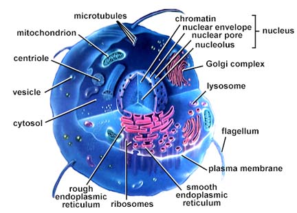
A model of a eukaryotic cell (picture
taken from On-Line Biology Book)
A eukaryotic cell has a nucleus, which is separated from the rest of the cell by a membrane. The nucleus contains chromosomes, which are the carrier of the genetic material (Section 3). There are internal membrane enclosed compartments within eukaryotic cells, called organelles, e.g., centrioles, lysosomes, golgi complexes, mitochondria among others (see picture above), which are specialised for particular biological processes. The mitochondria are found in all eukaryotes and are specialised for energy production (respiration). Chloroplasts are organelles found in plant cells which produce sugar using light. Light is the ultimate source of energy for almost all life on Earth. The area of the cell outside the nucleus and the organelles is called the cytoplasm. Membranes are complex structures and they are an effective barrier to the environment, and regulate the flow of food, energy and information in and out of the cell. There is a theory that mitochondria are prokaryotes living within eukaryotic cells.
An essential feature of most (prokaryote and eukaryote) living cells is their ability to grow in an appropriate environment and to undergo cell division. The growth of a single cell and its subsequent division is called the cell cycle. However, not all cells continually grow and divide, for example neurons only undergo an initial growth phase. Prokaryotes, particularly bacteria, are extremely successful at multiplying - it is likely that natural selection has favoured single celled organisms able to grow and divide quickly. Multicellular organisms typically begin life as a single cell, usually as a result of fusion of a male and a female sex cell (gametes). The single cell has to grow, divide and differentiate into different cell types to produce tissues and in higher eukarotyes, organs. Cell division and differentiation need to be controlled. Cancerous cells grow without control and can go on to form tumours. Development of single cells into complex organisms is in itself an area of study called developmental biology. This year’s Nobel prize for Physiology or Medicine has been awarded to scientists for the discoveries of key regulators of the cell cycle.
Cells consist of molecules.
2. Molecules of life
There are four basic types of molecules involved in life: (1) small molecules, (2) proteins, (3) DNA and (4) RNA. Proteins, DNA and RNA are known collectively as biological macromolecules.
2.1. Small molecules
These can be the building blocks of the macromolecules or they can have independent roles, such as signal transmission or being a source of energy or material for a cell. Some important examples besides water are sugars, fatty acids, amino acids and nucleotides. For instance, biological membranes are constructed from fatty acids, into which macromolecules are embedded. There are 20 different amino acid molecules, which are the building blocks for proteins (to be more precise, there are 19 amino acids and one which has a slightly different structure and therefore is called imino acid).
(Image taken from the On-Line Biology Book)
These are three examples of amino acid moleclues, there are 17 more. They differ by R side chains which determine their properties and the order of these different amino acids within the protein determines the three dimensional structure of the protein. There is a convention that each amino-acid is denoted by a letter in Latin alphabet, for instance arginine is denoted by R, histidine by H, lysine by L and there are 20 such letters.
2.2 Proteins
Proteins are the main building blocks and functional molecules of the cell, taking up almost 20% of a eukaryotic cell’s weight, the largest contribution after water (70%). Among others, there are
- Structural proteins, which can be thought of as the organism's basic building blocks. An example is collagen, which is the major structural protein of connective tissue and bone.
- Enzymes, which perform (catalyse) a multitude of biochemical reactions, such as altering, joining together or chopping up other molecules. Together these reactions and the pathways they make up is called metabolism. For example the first step in the glycolysis pathway, which is the conversion of glucose to glucose 6-phosphate, is catalysed by the enzyme hexokinase. Usually enzymes are very specific and catalyse only a single type of reaction, however the same enzyme can play role in more than one pathway.
- Transmembrane
proteins are key in maintenance of the cellular environment, regulating cell
volume, extraction and concentration of small molceules from the extracellular
environment and generation of ionic gradients essential for muscle and nerve
cell function. An example is the sodium/potassium pump.
Proteins have
complex three dimensional (3D) structure (see figure below). Four levels of
protein structure are distinguishable:
- Proteins are chains of 20 different types of amino acids, which in principle can be joined together in any linear order, sometimes called poly-peptide chains. This sequence of amino-acids is known as the primary structure, and it can be represented as a string of 20 different symbols (i.e., a word over the common alphabet of 20 letters). Information about various protein sequences and the functional roles of the respective proteins, can be found in UniProtKB/Swiss-Prot database. UniProtKB/Swiss-Prot is a joint project between the EBI and the Swiss Institute of Bioinformatics (SIB). The length of the protein molecule can vary from few to many thousands of amino-acids. For example insulin is a small protein and it consists of 51 amino acids, while titin has ~28,000 amino acids.
- Although the primary structure of a protein is linear, the molecule is not straight, and the sequence of the amino acids affects the folding. There are two common substructures often seen within folded chains - alpha-helices and beta-strands. They are typically joined by less regular structures, called loops. These three are called secondary structure elements.
- As the result of the folding, parts of a protein molecule chain come into contact with each other and various attractive or repulsive forces (hydrogen bonds, disulfide bridges, attractions between positive and negative charges, and hydrophobic and hydrophilic forces) between such parts cause the molecule to adopt a fixed relatively stable 3D structure. This is called tertiary structure. In many cases the 3D structure is quite compact.
- A protein may be formed from more than one chain of amino-acids, in which case it is said to have quaternary structure. For example haemoglobin, is made up of four chains each of which is capable of binding an iron molecule.
Proteins are much too small to be seen in an optical microscope - a characteristic protein size varies from about 3 to 10 nanometers (nm), i.e., 3 to 10 times 10-9 m, and solving (i.e., discovering) their structure is a difficult and expensive exercise (approximately €50,000 - €200,000 per novel structure), which is done by a variety of methods including X-ray crystallography, nuclar-magnetic resonance spectroscopy, and advanced electron microscopy. MSD is a database of known protein structures, which is housed and developed at the EBI. The images below shows the structure of triosephosphate isomerase visualised by RasMol software package, a 3D viewer for MSD structures.
In this image the
magenta coloured bits are alpha-helices, while yellow bits are
beta-strands.
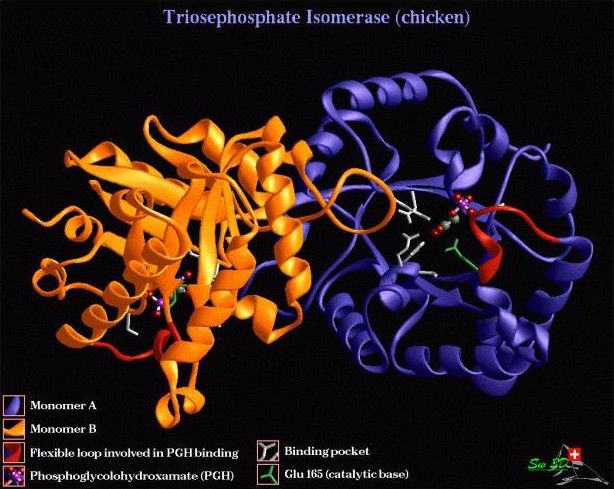
An alternative view in which the two monomer units are highlighted.
The size of this protein in a crystallised state is about 13 x 7 x 5 nm. The images above are only models of these molecules, as the molecules are two small to have a ‘real’ image. For instance they cannot have any conventional colour, they are in constant motion, and when we start zooming in into a finer structure, quantum effects, such as Heisenberg uncertainty principle start playing role.
There are roughly 15,000 protein structures deposited in public databases, though many of them are very similar to each other. Whether to consider two protein structures similar or different depends on the similarity threshold (as with cell types). Structural biologists think that currently there are about 1,500 different representative protein structures known.
All four structural levels are essentially determined by the primary structure (i.e., the amino-acid sequence) plus the physico-chemical environment where the molecule is placed. Predicting protein structure from the amino-acid sequence is one of the most important problems of computational biology (another name for bioinformatics, though some try to make a distinction between these two terms) and is far from being solved. Characteristic, frequently reoccurring structural elements are called protein domains. Sometimes it is possible to identify these domains in proteins of unknown structure, if their sequence is similar to that of a known structural domain. Structural domains are often associated with a particular protein function. Protein similarity is also deemed to be the result of evolutionary relationship.
What are the comparative sizes of proteins and cells? There is a proverb saying that size does not matter. Still comparative sizes may matter, particularly if we try to imagine the cellular processes described in the next sections. A typical linear dimension (diameter) of a globular protein is about 5 x 10 -9 m, while of a eukaryotic cell about 5 x 10 -5 m. This means the a cell is about a 10,000 times larger than a protein linearly. Alternatively, if we estimate the average weight of a human cell as about 10 -9 g, and remember that proteins constitute about one fifth of cell mass, then assuming the weight of an average protein to be about 10 -19 g (say hemoglobin is 64,500 atomic units, each of which is 1.66 x 10 -24 g), we see that there are 0.2 x 10 -9 / 10 -19 proteins per cell, which equals two billion (2 x 10 9 ). These of course are very rough estimates which would vary from cell to cell. If we remember that there are about 6 x 10 13 cells, we see that there are 30,000 times more cells per human, than proteins per cell. This may be an indication of the relative complexity of a human compared to a single cellular organism (a similar estimate regarding the relative complexity of an elephant or dinosaur and human may not be flattering for a human).
Although forces such as hydrogen bonds are weak individually, when two or more biological macromolecules with complementary shapes come close to each other, the sum of all such weak forces may cause the molecules interact rather strongly, e.g., to make them stick together. In fact, such weak inter-molecular forces and interactions play a fundamental role in life and are at the basis of virtually all biological processes. For instance many proteins can stick together to form large protein complexes such as yeast RNA polymerase II, which reads and transcribes the genetic information (see Section 3.3), and which has 10 subunits and for which the structure has been solved recently. These weak interactions also underlie how microarrays work, which is discussed in the last section.
2.3. DNA
DNA is the main information carrier molecule in a cell. DNA may be single or double stranded. A single stranded DNA molecule, also called a polynucleotide, is a chain of small molecules, called nucleotides . There are four different nucleotides grouped into two types, purines: adenosine and guanine and pyrimidines: cytosine and thymine. They are usually referred to as bases (in fact bases are the only distinguishing element between different nucleotides, see figure below) and denoted by their initial letters, A,C ,G and T (not to be confused with amino acids!).
(picture taken from
On-Line Biology Book )
Different nucleotides can be linked together in any order to form a
polynucleotide, for instance, like this
A-G-T-C-C-A-A-G-C-T-T
Polynucleotides
can be of any length and can have any sequence. The two ends of this molecule
are chemically different, i.e., the sequence has a directionality, like this
A->G->T->C->C->A->A->G->C->T->T->
The end of the polynucleotide are marked either 5' and 3' (this has chemical reasons
in the numbering of the –OH groups of the sugar ring); by convention DNA is
usually written with 5' left and 3' right, with the coding strand at top. Two
such strands are termed complementary , if one can be obtained from the
other by mutually exchanging A with T and C with G, and changing the direction
of the molecule to the opposite. For
instance,
<-T<-C<-A<-G<-G<-T<-T<-C<-G<-A<-A
is complementary to the
polynucleotide given above. Specific pairs of nucleotides can form weak
bonds between them. A binds to T, C binds to G (to be more precise, two hydrogen
bonds can be formed between each A-T pair, and three hydrogen bonds between each
C-G pair). Although such interactions are individually weak, when two longer
complementary polynucleotide chains meet, they tend to stick together, like
this
C-G-A-T-T-G-C-A-A-C-G-A-T-G-C
| | | | | | | | | | | | | | |
G-C-T-A-A-C-G-T-T-G-C-T-A-C-G
Vertical
lines between two strands represent the forces between them (to be more accurate
we could draw triple lines between each C and G and double lines between A and
T) as shown below. The A-T and G-C pairs are called base-pairs (bp). The
length of a DNA molecule is usually measured in base-pairs or nucleotides (nt),
which in this context is the same thing.
(picture taken from the
On-Line Biology Book )
Two complementary polynucleotide chains form a stable structure, which resembles a helix and is known as a the DNA double helix. About 10 bp in this structure takes a full turn, which is about 3.4 nm long.
(picture taken from the On-Line
Biology Book )
This structure was first figured out in 1953 in Cambridge by Watson and Crick (with the help of others), and the birthplace of this structure is often thought to be the Eagle pub on Bene't street. Later they got the Nobel Prize for this discovery, for more see the book by Watson – The Double Helix.
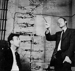
Watson and Crick at their DNA model molecule
It is remarkable that two complementary DNA polypeptides form a stable double helix
almost regardless of the sequence of the nucleotides. This makes the DNA
molecule a perfect medium for information storage. Note that as the strands are
complementary, each one of them fully determining the other, therefore for the
information purposes it is enough to give only one strand of the genome
molecules. Thus, for many information related purposes, the molecule used on the
example above, can be represented as CGATTCAACGATGC. The maximal amount of
information that can be encoded in such a molecule is therefore 2 bits times the
length of the sequence. Noting that the distance between nucleotide pairs in a
DNA is about 0.34 nm, we can calculate that the linear information storage
density in DNA is about 6x10 8 bits/cm, which is approximately 75 GB
or 12.5 CD-ROMs per cm.
Complementarity
of two strands in the DNA is exploited for copying (multiplying) DNA molecules
in a process known as the DNA replication, in which one double stranded DNA is replicated into two identical ones.
(The DNA double helix unwinds and forks during the process, and a new
complimentary strand is synthesised by specific molecular machinery on each
branch of the fork. After the process is finished there are two DNA molecules
identical to the original one.)
In a cell this happens during the cell division (see Section 1) and a
copy identical to the original goes to each of the new cells.
Note that mismatched components between polynucleotide strands are possible, if the total
sum of weak forces between the complementary nucleotides are strong enough. So
the molecules like
C-G-A-T-T-G-C-C-A-C-G-A-T-G-C
| | | ~ | | | ~ | | | ~ | | |
G-C-T-T-A-C-G-T-T-G-C-A-A-C-G
are
chemically possible, though they may be rare in a living cell. More bonds, i.e.,
more complementary pairs, makes the molecule more stable. If there are not
enough bonds, the two stranded molecular structure may become weak and the
strands may come apart. The number of links needed to keep the double-helix
together depends on the temperature (so-called melting temperature) and other
environmental factors. DNA which is no longer in the helical form is said to be
denatured.
2.4. RNA
RNA like DNA is constructed from nucleotides. But instead of the pyrimidine thymine (T), it has an alternative uracil (U), which is not found in DNA. Because of this minor difference RNA do not form a double helix, instead usually they are single stranded, but may have complex spatial structure due to complementary links between the parts of the same strand (as for instance in tRNA, section 4.2). RMA has various functions in a cell, some of them discussed in the next section, e.g., mRNA and tRNA are functionally different types of RNA which are both required for protein synthesis discussed in section 3.3.
RNA can bind complementary to a single strand of a DNA molecule, even though T is
replaced by U, so molecules like this
C-G-A-T-T-G-C-A-A-C-G-A-T-G-C
| | | | | | | | | | | | | | |
G-C-U-A-A-C-G-U-U-G-C-U-A-C-G
are possible and in fact play an important role in life processes and in
biotechnology.
There is a hypothesis that the first life on earth may have been RNA based. RNA can encode genetic information, is replicable, forms complex 3D structures and can also act as a catalyst for certain chemical reactions related to splicing (see section 3.3).
3. Genes and genomes
3.1 Chromosomes, genomes and sequencing
In a typical cell there are one or several long double stranded DNA molecules organised as chromosomes. In eukaryotes chromosomes have a complex structure where DNA is wound around structural proteins called histones. A human has 23 pairs of chromosomes , which are large enough to be seen in an optical microscope. The total length of the DNA in one human cell, if we could stretch it out, would be more than 1m. Mitochondria (section 1) contain DNA too, but the amount is minuscule in comparison to chromasomal DNA. Chromasomal and mitochondrial DNA forms the genome of the organism. All organisms have genomes and they are believed to encode almost all the hereditary information of the organism. In eukaryotes chromosoms are in the nucleus (apart from mitochondrial genomes), contained by the nuclear membrane. All cells in an organism contain identical genomes (with few rather special exceptions), as the result of DNA replication at each cell division.
There is a molecular machinery in cells, which keeps both DNA strands intact and complementary (i.e., if one strand is damaged, it is repaired using the second as a template). This is important as DNA damage (caused by environmental factors like radiation) can result in breaks in one or both strands, or mispairing of the bases, which would disrupt DNA replication among other things. If damaged DNA is not repaired the result can be cell death or tumours. Changes in genomic DNA are known as mutations.
The total genome size differ quite considerably in different organisms, as given in the table below.
|
Organism |
Number
or |
Genome size
in |
|
1 |
~400,000 - ~10,000,000 | |
|
12 |
14,000,000 | |
|
6 |
100,000,000 | |
|
4 |
300,000,000 | |
|
5 |
125,000,000 | |
|
23 |
3,000,000,000 |
Note that these sizes determine the upper bound of the genetic information in the organism.
Determining the four letter sequence for a given a DNA molecule is known as the DNA sequencing. The first full genome for a bacterium was sequenced in 1995. The yeast (Saccharomyces cerevisiae) genome was sequenced in 1997, worm (nematode Caenorhabditis elegans) in 1999, fly (Drosophila melanogaster) in 2000, and weed (Arabidopsis thaliana ) at 2001. About 90% or so of the human genome was completed in 2001, this is known as the draft human genome.
Sequencing of the relatively small bacterial genomes has become routine and is largely done by sequencing robots and completed by human researchers, the main problem being the minimisation of costs per letter, and maximisation of the speed while maintaining quality. Sequencing of larger genomes, like a human genome, is still difficult, though most of the problems are computational. Sequencing robots are able to sequence only relatively short stretches of DNA, which afterward have to be assembled together by a computer using assembly algorithms. The main difficulty is that genomes of higher eukaryotes (like humans) have many repeated subsequences, which makes the assembly rather tricky, this means that considerable human intervention is still needed in the final stage of sequencing projects.
The worlds largest public genome sequencing project is housed at the Sanger Institute (the large building next to the EBI). It is obvious, that because of the size of even the smallest bacterial genomes, the genome sequencing would not make much sense unless the sequences were stored in computer databases, allowing automatic search, comparison and other analyses. All the public DNA sequences (including the completed genomes) are stored in the EMBL database (also known as EMBL-Bank), which is in fact a collaboration of three databases EMBL in Europe, GenBank in the USA and DDBJ in Japan (each database mirrors the others and they exchange data every 24 hours).
The sequences contained in EMBL can be used as a resource to compare newly sequenced stretches of DNA. If a similar sequence is already in the EMBL database we can sometimes infer a biological function by analogy. Sequence comparison can be done by dynamic programming algorithms, but heuristic comparison algorithms, for instance FASTA and BLAST are more popular because of speed.
Genomes contain genes, most of which encode proteins.
3.2 Mendel, peas and classical genetics
Genetics started in the 19th century without any knowledge about DNA. Gregor Mendel bred peas in his garden and noticed that the inheritance sometimes follows clear rules. For instance if we cross peas which have green and yellow seeds, while in the next generation all seeds will be yellow, two generations later one quarter of the seeds will be green, while three quarters will be yellow. To explain this Mendel introduced the notion of dominant (yellow in our example) over the recessive (green) properties and the notion of gene (though he did not use this name yet) – the carrier of inheritance. This was before the discovery of chromosomes. Later, but before the DNA structure was discovered, it was correctly hypothesized that genes are located in chromosomes.
Not all inheritable properties are so simple. Crossing of some plants with red and white flowers can have a daughter generation with pink flowers. There is a lot more fun stuff in this area of research, which is usually termed classical genetics. This is a typical black box approach to biology - study the external properties of a biological system and guess at a mechanism to explain this. It become known only in the second half of the 20th century that DNA is the carrier of genes, and that this information is passed from generation to generation by DNA replication.
3.3 Genes and protein synthesis
There are many discussions between biologists to find a comprehensive definition of a gene, which is not easy, if possible at all. For our purposes
| A gene is a continuous stretch of a genomic DNA molecule, from which a complex molecular machinery can read information (encoded as a string of A, T, G, and C) and make a particular type of a protein or a few different proteins. |
This “definition” is not precise, and to better understand it we need to describe the molecular machinery making proteins based on the information encoded in genes. This process is called protein synthesis and has three essential stages: (1) transcription, (2) splicing, and (3) translation.
1. In transcription phase one strand of DNA molecule is copied into a complementary pre mRNA (pre stands for preliminary and m for messenger) by the protein complex RNA polymerase II (see section 2.2 and 2.4). In the process the two-stranded DNA double helix is unwound and information is read only from one strand (sometimes called the W-strand).
2. Splicing removes some stretches of the pre mRNA, called introns, the remaining sections called exons are then joined together. Note that the removal of introns is a consequence of the way how eukaryote genomes are organised. The genomic DNA that corresponds to the coding part of genes is not continuous, but consists of exons and introns. Exons are the part of the gene that code for proteins and they are interspersed with non coding introns which must be removed by splicing. The number and size of introns and exons differs considerably between genes and also between species. Only very few genes in yeast have introns, while for human threre are about 4 introns per gene on average, and the average size of exons is 150 bp and just above 3400 bp for introns. Prokaryote genes do not have introns and the splicing step is not present. The result of splicing is mRNA. Many eukaryote genes are known to have different alternative splice variants, i.e. the same pre-mRNA producing different mRNAs, known as alternative splicing.
(picture taken from On-Line
Biology Book )
Translation is the process of making proteins by joining together amino acids in order encoded in the mRNA. The order of the amino acids is determined by 3 adjacent nucleotides (triplets) in the DNA. This is known as the triplet or genetic code . Each triplet is called a codon and codes for one amino acid. As there are 64 codons and only 20 amino acids the code is redundant, for example histidine is encoded by CAT and CAC. In cytoplasm the mRNA forms a complex with ribosomes, which are large complexes of proteins and RNA molecules. The precise interactions and functions of all protein in ribosomes are not yet fully understood.
(picture taken from On-Line Biology Book)
Different transfer or tRNA molecules each carries one specific amino acid to the ribosome and specifically recognises one codon on the mRNA. The amino acid carried by the tRNA is added to the nascent (growing) protein. The translation is a complex process and not all the details are understood. Luckily most of these details are not crucial for understanding of bioinformatics. What is crucial however is to realise that there is nothing magical about proteins synthesis.
The end of translation is the final part of gene expression and the final product is a protein, the sequence of which corresponds to the sequence encoded by the mRNA. Proteins can be post-translationally modified e.g., by adding of sugars or cleavage (chopping), and this affects their location and function.
Biologists used to believe in paradigm - 'one gene - one protein'. Now this is known not to be true - due to alternative splicing and post-translational modifications one gene can produce a variety of proteins. There are also genes that do not encode proteins but encode RNA (for instance tRNA and ribosomal RNA).
3.4 Gene prediction, counting, annotation, ENSEMBL and UniProtKB/TrEMBL
It is an interesting question: given the genomic DNA sequence, can we tell where the genes are? The answer is that we can, although the accuracy of such predictions is not very high. Most of the knowledge to do these predictions comes from experimentally identified genes. There are about 6700 experimentally confirmed genes in the human genome (to be more accurate - 6700 experimentally verfied cDNAs). Gene prediction is an important problem for computational biology and there are various algorithms that do gene prediction using known genes as a training data set. A popular algorithmic technique used in gene prediction are hidden Markov models (HMMs).
Even if we knew where the genes are in the genome, it is not entirely obvious how to count them. Due to the existence of overlapping genes and splice variants it is difficult to define which parts of the DNA should be regarded as the same or several different genes. Nevertheless, for practical purposes (allowing for some 'experimental error') we can count how many genes an organism has. Some of the results of counting of predicted genes have turned out to be quite surprising.
| Organism | The number of predicted genes |
Part of the genome that encodes proteins (exons) |
| E. coli (bacteria) | 5000 | 90% |
| yeast | 6000 | 70% |
| worm | 18,000 | 27% |
| fly | 14,000 | 20% |
| weed | 25,500 | 20% |
| human | 30,000 | 5% |
One of the surprises is the relatively small number of genes in a human genome in comparison to worm. Before most of the human genome sequencing was accomplished, it was estimated that there should be about 100,000 genes in a human. In fact some experts still think that there must be at least 40,000 - 50,000 genes in the human genome, and that 30,000 just reflects the unreliability of in silico (i.e., computational) gene prediction. Still, it seems that there is no simple correlation between the intuitive (not well-defined) complexity of an organism and the number of genes in its genome (for instance, intuitively fly is more complex organism than worm ). One reason for the low number of genes in the human genome may be that there are more splice variants per gene in humans, though this has yet to be proved (otherwise human vanity may have to suffer).
The presence of 95% of non-coding DNA in the human genome (sometimes called the junk DNA) remains a mystery. There are several hypotheses explaining this, but none is generally accepted. One controversial hypothesis (promoted by Richard Dawkins) is based on the idea of so-called selfish DNA. It states that the DNA is the basic element for natural selection, implying that DNA tries to propagate (multiply and amplify) itself, while the cells and organisms are vehicles to achieve this.
Automated gene prediction has been critical in making sense of the unfinished or draft data from genome projects. Sequence data is assembled into larger pieces (contigs), related to known genetic markers on chromosomes to order them and the gene predictions can then be placed on the unfinished sequence. The ENSEMBL project offers annotation for gene prediction in eukaryotes. ENSEMBL is a joint project between the EBI and the Sanger Institute.
Currently most new entries to UniProtKB/Swiss-Prot database come from UniProtKB/TrEMBL, which are automatically translated DNA sequences of predicted genes in EMBL database into protein sequences.
3.5 Genome similarity, SNPs and comparative genomics
Those who are learning about genome sequencing for the first time often ask the question - whose genome is being sequenced? Is it a particular individual? This is not an unreasonable question, in fact several anonymous samples were collected and pooled for the human genome project. But this does not really matter as all human genomes are deemed to be roughly 99.9% equivalent and on average one in a thousand nucleotides are different in genomes of two different individuals. Therefore we can talk in terms of the consensus human genome.
The 0.1% difference is exploited in DNA fingerprinting used in criminology. Variations in non-coding parts of the genome are analysed to produce patterns that can reliably distinguish individuals, an exception here is identical twins which are much harder to distinguish with DNA fingerprinting.
Particularly important variations in individual genomes are the single nucleotide polymorphisms or SNPs, which can occur both in coding and non-coding parts of the genome. SNPs are DNA sequence variations which occur when a single base (A,C,G, or T) is altered so that different individuals may have different letters in these positions. Particular nucleotides in SNP positions within or close to genes can influence the gene's protein product. Some 'abnormal' protein variants (mutant variants) are the cause of genetic diseases. SNPs may be responsible for many inheritable differences between individuals, and SNP variation may indicate the predisposition to a genetic disease. For example there is evidence that certain combinations of SNPs occur in individuals with Alzheimers disease. SNP analysis is therefore important for diagnostics and a SNP database is being built with the participation of the EBI. SNP analysis can also be used in population genetics, as some SNPs vary in frequency between populations. There are about 3 million SNPs collected in public SNP databases.
The sequencing projects have revealed that the genomes of what look like very different organisms may be quite similar. An example of this is similarity between yeast and worm described in the next section. It is estimated that the difference between human and chimpanzee genomes is only 1-3%, while between human and mouse only about 5% - 15%, depending on how the similarity is defined and measured (before the sequencing of chimp and mouse are well under way, these are only estimates). These similarities indicate close evolutionary relationships between these mammalian organisms. It is possible to build a phylogenetic tree of the evolution of proteins, genes and organisms based on sequence comparisons.
4. Functional genomics
Functional genomics can be roughly defined as using the emerging knowledge about genomes to understand the gene and their product functions and interactions, and most importantly of all, how all this makes organisms to function the way they do.
4.1 Gene functions and GO
As we already mentioned, proteins play a variety of roles in a cell. Biologists think that there is likely to be a limited universe of genes and their respective proteins, from the functional point of view, many of which are present in most or all genomes. For instance, about 12% of the ~18 000 worm genes encode proteins whose biological roles could be inferred from their sequence similarity to yeast genes, and vice versa - almost a third of the ~6000 yeast genes have functional equivalents in worm genes. The recognition of the limited universe of genes has prompted unification of biology under the name Gene Ontology or GO.
The aim of the GO project is the development of a dynamic controlled vocabulary for description of gene function and localisation. GO works at three levels for each gene product: molecular function, biological process and cellular component. The vocabulary is organised in three independent directed acyclic graphs (DAG's) characterising the genes at each of these three levels. The use of GO terms allows automated searching of gene function in databases. Proteins in UniProtKB/Swiss-Prot and the Interpro databases (another project at the EBI that classifies proteins by a variety of computational methods) are currently being assigned GO terms.
4.2 Protein abundance in a cell
Proteins in a cell are synthesised from genes and their life cycle can be roughly described as synthesis, functionality and degradation. Nobody really knows how many different proteins are synthesized from the estimated 30,000 genes in a human cell. Due to alternative splicing and post-translational modifications this number apparently is much higher than the number of genes. Evidently, not all the proteins have to be present in a given cell at a given moment.
The protein abundance may depend on many factors such as whether the respective gene is expressed (i.e., is actively transcribed) or not, how intensively (how fast) it is expressed, whether and how fast it is spliced, translated and modified, how long a half-life the mRNA and the protein have, and whether it is actively degraded at a given moment. Direct experimental studies of protein abundance are technically difficult at present. However, thanks to the microarray technology (see next section), it is possible to measure the mRNA abundance (gene expression) for tens of thousands of genes in parallel in a single experiment. The correlation between gene expression and the presence of the respective proteins in the cell is not straightforward, still, in many cases some estimates about the proteins can be made from gene expression.
There is evidence that for most of the 320 different cell types in a human body, only about 10%-20% of the genes are expressed in any particular state or developmental stage. These numbers are not very reliable as the studies are difficult and some gene products may have very low abundance levels, which may be difficult to detect experimentally.
Another question related to protein abundance in a cell is which proteins interact with which at some point in cell's life. This is known as protein-protein interaction networks. There is a plan to build a protein-protein interaction database at the EBI and there is work going on at the EBI to predict such interactions by computational methods.
4.3 Gene regulation and networks
Another important and interesting question in biology is how gene expression is switched on and off, i.e., how genes are regulated. Since almost all cells in a particular organism have an identical genome (section 3), differences in gene expression and not the genome content are responsible for cell differentiation (how different cell types develop from a fertilised egg) during the life of the organism.
Gene regulation in eukaryotes, is not well understood, but there is evidence that an important role is played by a type of proteins called transcription factors. The transcription factors can attach (bind) to specific parts of the DNA, called transcription factor binding sites (i.e., specific, relatively short combinations of A, T, C or G), which are located in so-called promoter regions. Specific promoters are associated with particular genes and are generally not too far from the respective genes, though some regulatory effects can be located as far as 30,000 bases away, which makes the definition of the promoter difficult.
Transcription factors control gene expression by binding the gene's promoter and either activating (switching on) the gene's transcription, or repressing it (switching it off). Transcription factors are gene products themselves, and therefore in turn can be controlled by other transcription factors. Transcription factors can control many genes, and some (probably most) genes are controlled by combinations of transcription factors. Feedback loops are possible. Therefore we can talk about gene regulation networks . Understanding, describing and modelling such gene regulation networks are one of the most challenging problems in functional genomics.
There are over 200 known transcription factors in yeast, over 600 in worm and fly, and over 1500 in weed, but the real numbers are probably higher, since more than half of the predicted genes in these organism have unknown function and there are transcription factors likely to be found among the unknown genes. In addition, transcription factors are not the only proteins participating in gene regulation - proteins affecting chromatine structure are another example, and it is know that at least some regulation is happening in the translation stage. Microarrays and computational methods are playing a major role in attempts to reverse engineer gene networks from various observations. Note that in reality the gene regulation is likely to be a stochastic and not a deterministic process.
Traditionally molecular biology has followed so-called reductionist approach mostly concentrating on a study of a single or very few genes in any particular research project. There is a proverb – ‘one gene at a time’ or ‘one post-doc, one gene’. With genomes being sequenced, this is now changing into so-called systems approach. We can begin asking questions such as how many genes are expressed in different cell types, which genes are expressed in all cell types, what are the functional roles of these genes, how big is the gene function universe, how many genes are needed for life, how it can be that a worm has more genes than a fly, and the human only a bit more than a worm, and, of course, we can always revisit the question of the meaning of life.
5. Microarrays and gene expression databases
Microarray technology makes use of the sequence resources created by the genome projects and other sequencing efforts to answer the question, what genes are expressed in a particular cell type of an organism, at a particular time, under particular conditions. For instance, they allow comparison of gene expression between normal and diseased (e.g., cancerous) cells. There are several names for this technology - DNA microarrays, DNA arrays, DNA chips, gene chips, others. Sometimes a distinction is made between these names but in fact they are all synonyms as there are no standard definitions for which type of microarray technology should be called by which name.
5.1 Microarray technology and applications
Microarrays exploit the preferential binding of complementary single-stranded nucleic acid sequences (see section 2.3-2.4). A microarray is typically a glass (or some other material) slide, on to which DNA molecules are attached at fixed locations (spots). There may be tens of thousands of spots on an array, each containing a huge number of identical DNA molecules (or fragments of identical molecules), of lengths from twenty to hundreds of nucleotides. (According to quick napkin calculations by Wilhelm Ansorge and John Quackenbush in Schnookeloch in Heidelberg on 4 October, 2001, the number of DNA molecules in a microarry spot is 107-108). For gene expression studies, each of these molecules ideally should identify one gene or one exon in the genome, however, in practice this is not always so simple and may not even be generally possible due to families of similar genes in a genome. Microarrays that contain all of the about 6000 genes of the yeast genome have been available since 1997. The spots are either printed on the microarrays by a robot, or synthesized by photo-lithography (similarly as in computer chip productions) or by ink-jet printing.
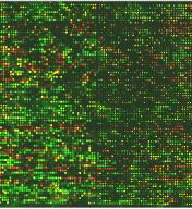
An illuminated microarray (enlarged). A typical dimension of such an array is about 1 inch or less, the spot diameter is of the order of 0.1 mm, for some microarray types can be even smaller.
There are different ways how microarrays can be used to measure the gene expression levels. One of the most popular micorarray applications allows to compare gene expression levels in two different samples, e.g., the same cell type in a healthy and diseased state (see figure below).
The total mRNA from the cells in two different conditions is extracted and labeled with two different fluorescent labels: for example a green dye for cells at condition 1 and a red dye for cells at condition 2 (to be more accurate, the labeling is typically done by synthesising single stranded DNA's that are complementary to the extracted mRNA by a enzyme called reverse transcriptase). Both extracts are washed over the microarray. Labeled gene products from the extracts hybridise to their complementary sequences in the spots due to the preferential binding - complementary single stranded nucleic acid sequences tend to attract to each other and the longer the complimentary parts, the stronger the attraction (see section 2.3 and 2.4).
The dyes enable the amount of sample bound to a spot to be measured by the level of fluorescence emitted when it is excited by a laser. If the RNA from the sample in condition 1 is in abundance, the spot will be green, if the RNA from the sample in condition 2 is in abundance, it will be red. If both are equal, the spot will be yellow, while if neither are present it will not fluoresce and appear black. Thus, from the fluorescence intensities and colours for each spot, the relative expression levels of the genes in both samples can be estimated.
The raw data that are produced from microarray experiments are the hybridised microarray images. To obtain information about gene expression levels, these images should be analysed, each spot on the array identified, its intensity measured and compared to the background. This is called image quantitation.
Image quantiation is done by image analysis software. To obtain the final gene expression matrix from spot quantiations, all the quantities related to some gene (either on the same array or on arrays measuring the same conditions in repeated experiments) have to be combined and the entire matrix has to be scaled to make different arrays comparable.
Gene expression monitoring is not the only microarray application, another one is SNP detection.
5.2 ArrayExpress
Microarray's are already producing massive amounts of data. These data, like genome sequence data, can help us to gain insights into underlying biological processes only if they are carefully recorded and stored in databases, where they can be queried, compared and analysed by different computer software programs. The EBI is currently establishing a public repository for microarray gene expression data ArrayExpress, analogous to EMBL-bank for DNA sequence data. In many respects gene expression databases are inherently more complex than sequence databases (this does not mean that developing, maintaining and curating the sequence databases are any less challenging).
Conceptually, a gene expression database can be regarded as consisting of three parts – the gene expression data matrix, gene annotation and sample annotation.
Gene expression data have meaning only in the context of the particular biological sample and the exact conditions under which the samples were taken. For instance, if we are interested in finding out how different cell types react to treatments with various chemical compounds, we must record unambiguous information about the cell types and compounds used in the experiments. EBI is participating in an effort to develop ontologies for sample annotation, this is analogous to gene ontology for gene description.
Gene annotation can be taken care to some extent of by links to sequence databases, unfortunately complicated many-to-many relationships between genes in the gene expression matrix and the features (spots) on the array makes it necessary to provide a full and detailed description of each feature on the array, as one gene can relate to several features on the array. The lack of standards in gene naming is another difficulty - a table relating each array feature present in the database to the list of all synonymous names of the respective gene is an essential part of a gene expression database.
The microarray technology is still rapidly developing, therefore it is natural that currently there are no established standards for microarray experiments and how the raw data should be processed. There are also no standard measurement units for gene expression levels. In the lack of such standards the information about how exactly the gene expression data matrix was obtained should be kept in the database, if the data are to be properly interpreted later. This complicates the data object model enormously.
ArrayExpress is storing all this information, the details of which is called Minimum Information About a Microarray Experiment (MIAME) defined by the Microarray Gene Expression Database (MGED) consortium. MGED is a grass roots movement that was founded at a meeting at the EBI in 1999, is supported by most of the important players in the microarray community, and has evolved far beyond the EBI.
An other repository for gene expression data GEO is being developed at NCBI in the US. DDBJ in Japan also have plans. All three groups face similar problems and are involved in MGED to some degree. A common data exchange format MAGE-ML is being developed in collaboration between MGED (with active participation of the EBI) and some major microarray companies.
6.3 Gene expression data analysis and Expression Profiler
Capturing and storage of microarray data is not an end in itself. The amounts of data from even a single microarray experiment are so large, that software tools have to be used to make any sense out of it. Clustering and class prediction are typical methods currently used in gene expression data analysis (see Microarray Data Analysis). One of the popular gene expression data analysis tools is Expression Profiler, developed at the EBI. The Microarray Informatics Team at the EBI is actively working in many microarray data analysis areas using this and other tools.
An example of such research is an approach to reverse engineering of gene regulatory networks, which is based on the hypothesis that genes that have similar expression profiles (i.e., similar rows in the gene expression matrix) should also have similar regulation mechanisms as there must be a reason why their expression is similar under a variety of conditions. Therefore, if we cluster the genes by similarities in their expression profiles and take sets of promoter sequences from genes in such clusters, some of these sets of sequences may contain a ‘signal’ as a specific sequence pattern such as a particular substring, which is relevant to regulation of these genes (see Mining for putative regulatory elements in the yeast genome using gene expression data).
There is much more exciting stuff going on at the EBI, to join click here.
Acknowledgements
- Wilhelm Ansorge (EMBL)
- Ewan Birney
- Gunars Brazma (University of Latvia)
- Midori Harris
- John Quackenbush (TIGR)
- JJ
- Alan Robinson
- Alphonse Thanaraj
- Caleb Webber
For questions and comments please contact the authors.
Further reading
- Nature - Human Genome Issue(Volume 409, p. 813-959, 2001).
- Science - Human Genome Issue (Volume 291, 2001)
- Nature Genetics - Chipping Forecast - devoted to microarrys (Volume 21 supplement 1-60, 1999)
- FEBS Letters - Functional Genomics (Volume 480, Nr. 1, August 2000)
Online resources
Textbooks on bioinformatics
- Teresa Attwood, David Parry-Smith, Introduction to Bioinformatics, Prentice Hall, 1999
- Dan Gusfield, Algorithms on Strings, Trees, and Sequences - Computer Science and Computational Biology, Cambridge University Press, 1997.
- Pavel Pevzner, Computational Molecular Biology - An Algorithmic Approach , The MIT press, 2000
Some other popular books
- Charles Darwin, The Origin of Species (theory of evolution)
- Richard Dawkins, The Selfish Gene (hypotheses of the selfish-DNA)
- Watson, D. J, The Double Helix; New York, London, W. W. Norton, 1980 (a personal account of the discovery of the structure of DNA)
Popular textbooks on molecular biology
(Molecular biology textbooks are typically rather big, but usually they mostly contain nice pictures through which one can learn a lot)
- Alberts, B. , Bray, D. , Lewis J., Raff, M., Roberts, K., Watson, J.D.: Molecular biology of the cell.
New York, Garland Publishing, 1994
Brown T. A.: Genetics; a molecular approach, London, Chapman & Hall, 1999 - Lewin B: Genes VII, New York, Oxford University Press, 2000
- Winter, P. C., Hickey, I. , Fletcher, H. L.: Instant Notes in Genetics, Oxford, 1998
Other references where some of the facts on this web-site are taken from
- Deutsch and Long, Intron-exon structures of eukaryotic model organism, Nuc Acids Res (27)15, 3119-3228, 1999
- Science (294) 81-121, 2001. Unlocking the genome - new developments in genomics